Grouped Tabsets Example

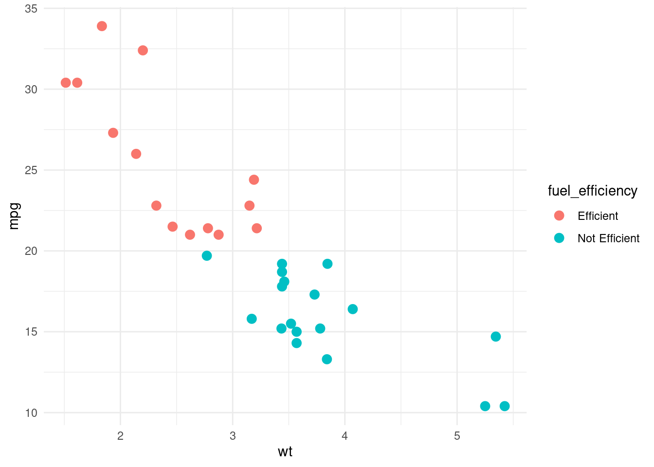
Here is an example of grouped tabsets in Quarto. Select Python to see both tabsets switch. The code is available on GitHub.

First tabset

R

library(ggplot2)
data("mtcars")
mtcars$fuel_efficiency <- ifelse(mtcars$mpg > 20, "Efficient", "Not Efficient")

mtcars |>
  ggplot(aes(x = wt, y = mpg, color = fuel_efficiency)) +
  geom_point(size = 3) +
  theme_minimal()

Python

import pandas as pd
from plotnine import ggplot, aes, geom_point, theme_minimal

mtcars = pd.read_csv("https://raw.githubusercontent.com/mwaskom/seaborn-data/master/mpg.csv").dropna()
mtcars['fuel_efficiency'] = ['Efficient' if mpg > 20 else 'Not Efficient' for mpg in mtcars['mpg']]

plot = (
    ggplot(mtcars, aes(x='weight', y='mpg', color='fuel_efficiency')) +
    geom_point(size=3) +
    theme_minimal()
    )

plot.show()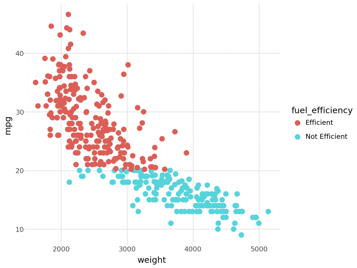

Second tabset

R

library(gt)
towny <- gt::towny

towny_mini <- towny[order(-towny$density_2021), c("name", "website", "density_2021", "land_area_km2", "latitude", "longitude")]
towny_mini <- head(towny_mini, 10)

gt(towny_mini)

name	website	density_2021	land_area_km2	latitude	longitude
Toronto	https://www.toronto.ca	4427.75	631.10	43.74167	-79.37333
Brampton	https://www.brampton.ca	2468.99	265.89	43.68833	-79.76083
Mississauga	https://www.mississauga.ca	2452.56	292.74	43.60000	-79.65000
Newmarket	https://newmarket.ca	2284.21	38.50	44.05806	-79.45833
Richmond Hill	https://www.richmondhill.ca	2004.39	100.79	43.87139	-79.43722
Orangeville	https://www.orangeville.ca	1989.91	15.16	43.91528	-80.10861
Ajax	https://www.ajax.ca	1900.75	66.64	43.85833	-79.03639
Waterloo	https://www.waterloo.ca	1895.66	64.06	43.46667	-80.51667
Kitchener	https://www.kitchener.ca	1877.68	136.81	43.41861	-80.47278
Guelph	https://guelph.ca	1644.06	87.43	43.53583	-80.22889

Python

from great_tables import GT, html
from great_tables.data import towny

towny_mini = (
    towny[["name", "website", "density_2021", "land_area_km2", "latitude", "longitude"]]
    .sort_values("density_2021", ascending=False)
    .head(10)
)

(
    GT(towny_mini)
)

name	website	density_2021	land_area_km2	latitude	longitude
Toronto	https://www.toronto.ca	4427.75	631.1	43.741667	-79.373333
Brampton	https://www.brampton.ca	2468.99	265.89	43.688333	-79.760833
Mississauga	https://www.mississauga.ca	2452.56	292.74	43.6	-79.65
Newmarket	https://newmarket.ca	2284.21	38.5	44.058056	-79.458333
Richmond Hill	https://www.richmondhill.ca	2004.39	100.79	43.871389	-79.437222
Orangeville	https://www.orangeville.ca	1989.91	15.16	43.915278	-80.108611
Ajax	https://www.ajax.ca	1900.75	66.64	43.858333	-79.036389
Waterloo	https://www.waterloo.ca	1895.66	64.06	43.466667	-80.516667
Kitchener	https://www.kitchener.ca	1877.68	136.81	43.418611	-80.472778
Guelph	https://guelph.ca	1644.06	87.43	43.535833	-80.228889